The spectral difference method has quite recently been proposed by Liu
et al. [8] and further developed
by Wang et al. [13] and
by the present authors [9]. Consider the
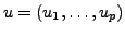
conservation law
![$\displaystyle \dd{u}{t} + \nabla \cdot F = 0 \ , \qquad (x,t) \in \Omega \times [0,T] \ ,$](img17.png) |
(1) |
subject to suitable initial and boundary conditions, where
 , and
, and
 , and the
divergence operation is to be taken componentwise for
, and the
divergence operation is to be taken componentwise for  .
The Spectral Difference method uses a pseudo-spectral collocation-based
reconstruction for both the dependent variables
.
The Spectral Difference method uses a pseudo-spectral collocation-based
reconstruction for both the dependent variables  and the flux
function
and the flux
function  inside a mesh element,
  , say.
Assume a triangulation of
, say.
Assume a triangulation of
 consisting of simplexes. The
reconstruction for the dependent variables can be written
consisting of simplexes. The
reconstruction for the dependent variables can be written
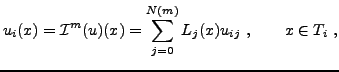 |
(2) |
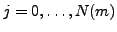
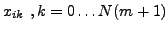
where
 , and
, and  is the
  solution
collocation node in the
solution
collocation node in the  mesh element (here and in the
following the double index notation refers to a node inside a
cell). The interpolation operator
mesh element (here and in the
following the double index notation refers to a node inside a
cell). The interpolation operator
 denotes a collocation
using polynomials of total degree
denotes a collocation
using polynomials of total degree  . The
. The  are the cardinal
basis functions for the chosen set of collocation nodes
are the cardinal
basis functions for the chosen set of collocation nodes  , where
 , and
, and  is determined by the chosen order of
accuracy. The reconstruction of the flux function in reads
is determined by the chosen order of
accuracy. The reconstruction of the flux function in reads
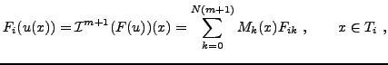 |
(3) |
where the  are the cardinal basis functions corresponding to the
collocation nodes
are the cardinal basis functions corresponding to the
collocation nodes
 , and
, and
 . If
the solution is reconstructed to order
. If
the solution is reconstructed to order  , the flux nodes are
interpolated to order
, the flux nodes are
interpolated to order  , because of the differentiation operation
in eq. (1). If the numerical flux is defined as the union
of all local interpolations, it will be discontinuous
at element boundaries. Instead we define the numerical flux function
, because of the differentiation operation
in eq. (1). If the numerical flux is defined as the union
of all local interpolations, it will be discontinuous
at element boundaries. Instead we define the numerical flux function  on
the triangle as
on
the triangle as
 |
(4) |
where the
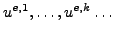 are ``external'' solutions on
triangles
are ``external'' solutions on
triangles  with
with
 such that
 , and
the value is given by
, and
the value is given by
 . For nodes
on edges of triangles there is only one external solution
. For nodes
on edges of triangles there is only one external solution  . It
is necessary for discrete conservation that the normal flux component
be continuous across the edge, which suggests one uses numerical flux
functions, standard in finite-volume formulations, such that the
normal flux component
. It
is necessary for discrete conservation that the normal flux component
be continuous across the edge, which suggests one uses numerical flux
functions, standard in finite-volume formulations, such that the
normal flux component
 , for the node
  , say, is
replaced by the numerical flux
, say, is
replaced by the numerical flux
 , where is the
edge normal, and
, where is the
edge normal, and  is the numerical flux function approximating
 . For flux nodes on corners of elements, one may compute the flux
using the numerical flux functions associated with both incident
edges, see [13]. For the numerical flux we
have used central average with both CUSP construction of artificial
diffusion [7] and simple scalar dissipation, as well
as Roe's approximate Riemann solver with good results.
. For flux nodes on corners of elements, one may compute the flux
using the numerical flux functions associated with both incident
edges, see [13]. For the numerical flux we
have used central average with both CUSP construction of artificial
diffusion [7] and simple scalar dissipation, as well
as Roe's approximate Riemann solver with good results.
Any combination of collocation
nodes may be used, provided that the nodes for  support a quadrature of the
order of the interpolation , and the restriction of the flux nodes to
the boundaries supports a
support a quadrature of the
order of the interpolation , and the restriction of the flux nodes to
the boundaries supports a  -dimensional quadrature of order
. This ensures discrete conservation in the sense that
is satisfied exactly for the solution and reconstructed flux
function [9].
For the solution nodes one can choose Gauss quadrature points.
Hesthaven proposed nodes based on the solution of an electrostatics
problem for simplexes [6] , which support both a
volume and a surface integration to the required degree of
accuracy. These nodes can be used for both flux and solution
collocation.
The baseline scheme is now readily defined in ODE form as
-dimensional quadrature of order
. This ensures discrete conservation in the sense that
is satisfied exactly for the solution and reconstructed flux
function [9].
For the solution nodes one can choose Gauss quadrature points.
Hesthaven proposed nodes based on the solution of an electrostatics
problem for simplexes [6] , which support both a
volume and a surface integration to the required degree of
accuracy. These nodes can be used for both flux and solution
collocation.
The baseline scheme is now readily defined in ODE form as
 ,
where the degrees of freedom are given by the values of the solution
at the collocation nodes,
,
where the degrees of freedom are given by the values of the solution
at the collocation nodes,
 , where again
is the solution collocation node in the mesh
element, and the right-hand side solution operator is given by the
exact differentiation of the reconstructed flux function:
, where again
is the solution collocation node in the mesh
element, and the right-hand side solution operator is given by the
exact differentiation of the reconstructed flux function:
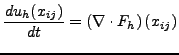 |
(5) |
Georg May
2006-02-23